Professor De Boer's list of
TEXTBOOK ERRATA
(last update 11/05/2018)
Alexander & Sadiku,
Fundamentals of Electric Circuits, 6th Ed.
ISBN 978-0-07-802822-9, McGraw-Hill, 2017.
(link to errata for the 5th edition.)
If you are considering purchasing this textbook and worrying that it is a poor choice due to the length of this list of errata, please don't worry about that. Competing textbooks have about as many errata, but perhaps no list like this. "Better the devil you know than the devil you don't." Professor De Boer likes this book enough to find it worthwhile to publish this list of errata.
The following errata have been found to date:When specific corrections are illustrated, additions are in blue text.
Deletions are instrikeout text. Commentary is in green text.
This file is under construction. A first pass effort has been done on the first twelve chapters. There are probably still more errors to be found, certainly in the later chapters. Some links may not be working right yet. One thing is clear. There are fewer errata in the 6th edition than there were in the 5th.
Page 4. Eight lines from the bottom of the page
schematic diagram for a radio transmitter
(Posted 8/23/2018 courtesy of e-mail from Jon H. Peterson.)
Page 10. Starting at the 3rd line just above Section 1.5
time-varying voltage is called an ac voltage and is represented by v. A
battery is typically a source of dc voltage. A generator is typically a source of ac voltage.
an electric generator.
There are many sources of dc voltage including some power supplies, solar cells, etc. Similarly, there are many sources of ac voltages including transducers, antennas, etc.
(Posted 8/23/2018 courtesy of e-mail from Jon H. Peterson.)
Page 16. Last paragraph on the page and Figure 1.17 on page 17
This paragraph is so far out-of-date as to be classified as errata. CRTs and iconoscopes (especially iconoscopes) are no longer in use. The interested reader may prefer to consult articles in Wikipedia to find modern background information on these topics. See especially Television Set and Video Camera Tube, and Charge Coupled Device. Otherwise, just ignore this paragraph in the textbook and Figure 1.17.
(Posted 8/23/2018 courtesy of e-mail from Jon H. Peterson.)
Page 17. The section labeled "Historical."
The statement that the CRT remains the most economical device today is out-of-date. By about 2010 flat-panel displays were decisively more economical than CRT displays. Also, with respect to television camera techniques this section only describes very early history (up to about 1960).
(Posted 8/23/2018 courtesy of e-mail from Jon H. Peterson.)
Page 42. Practice Problem 2.7, Figure 2.26
The label on the arrow near the 2 Ω resistor is incorrect. Delete the "over 3" portion of the label so that it is simply io. A corrected figure is shown below.
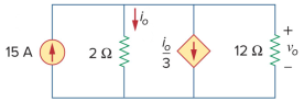
(Posted 8/23/2018 courtesy of e-mail from Jon H. Peterson.)
Page 49. Practice Problem 2.11
To get the answer shown, change the 6 S conductor the lower right position in Figure 2.41 to 8 S. Alternatively, the correct answer (to four significant figures) given Figure 2.41 with a 6 S conductor in the lower right position is 7.765 S."
(Posted 1/10/2017.)
Page 102. Practice Problem 3.9
In the 5 x 5 matrix, each instance of "–40" should be changed to "–20"
(Posted 1/05/2017.)
Page 103. About 1/3 of the way down the page
Mesh analysis is not the only way to analyze a transistor circuit. Loop analysis (not covered in this textbook), superposition, and various other techniques may be applied. Change the text as follows:
mesh analysis is
The interested reader may find a simplified presentation of the loop current method at Kahn Academy. A complete presentation of the loop current method requires the application of graph theory to assure a linearly independent set of equations. Such a presentation can be found in some older textbooks, for one example,
Gene H. Hostetter, Enginerring Network Analysis, Harper & Row Publishers, New York, 1984, ISBN 0-06-042907-0, p82-86.
(Posted 2/23/2018.)
Page 103. The paragraph just above Example 3.10 and other nearby text
The content of Appendix D from the 5th edition of this textbook has been moved to McGraw Hill's "Online Learning Center" called Connect for the 6th edition. The comment in the right-hand column of page 103 and Example 3.10 also should be edited to redirect the reader from "Appendix D" to the tutorial on McGraw Hill's "Connect" website.
The reader is expected to review Sections D.1 through D.3
Page 108. Example 3.12, first equation in the solution
A zero is missing. The "20" should be "200." The correrct equation is. . .
–4 + IB(200 × 103) + VBE = 0
(Posted 8/27/2018 courtesy of e-mail from Jon H. Peterson.)
Page 110. Practice Problem 3.13
The printed answers are wrong. Change them to
Answer:
Page 117. Problem 3.34
As printed, what is being requested is not precisely clear, especially for students who are learning the concept of a planar circuit. Change the problem statement so that it reads as follows:
For each
(Posted 1/05/2017.)
Page 247. Problem 6.64, Part (a) and Figure 6.86
As printed, the problem cannot be solved using techniques from Chapters 1 through 6. Change part (a) of the problem statement so that it reads as follows:
(a) i(t) for
Also, an incorrect symbol for the make-before-break switch is used in Figure 6.86 and the general order of flow of ideas from right-to-left in the textbook's schematic is counter-intuitive. A better schematic of the exact same circuit with a correct symbol for the switch and with the flow of ideas arranged from left-to-right is shown below.
![[image file not found]](IMG_4598_Figure_6p86page247_cropped_edited_web.png)
(Posted 2/23/2018, updated 2/24/2018.)
Page 303. Problem 7.28
An extra "(t)" appears near the end of the given function for i(t).
What is shown as u(t)(t – 4) should be u(t – 4). Correct it as follows:
i(t) = [r(t) – r(t – 1) – u(t – 2) – r(t – 2)
+ r(t – 3) + u
(Posted 3/01/2017.)
Page 337. Practice Problem 8.8
The answers printed, are wrong. Change them as follows:
Answer:
(Posted 3/01/2017.)
Page 357. Problem 8.5
The first derivative in part (b) is printed wrong. Change it as follows;
(b)
(Posted 4/19/2017.)
Page 469. Definition of Power Factor
Change the definition as follows:
The power factor is the ratio of the real power to the apparent power.
Change the nearby sidebar text as follows:
From Eq. (11.36) the power factor may also be regarded as the cosine of the phase angle of the voltage with respect to the phase angle of the current, or (from Eq. 11.39) as the cosine of the angle of the load impedance.
A definition must be the most broadly useful statement possible, in this case to include non-sinusoidal voltages and currents too. One can then note that for sinusoidal steady state conditions, Equations 11.36 and 11.39 imply that the power factor can be found from the cosine of the angle between voltage and current or the cosine of the angle of the load impedance.
(Posted 1/28/2017)
Page 472. Equation 11.48
The "I" should be italicized. Change it as follows from:
P = Re(S) = I2
rmsR to
P = Re(S) = I2
rmsR
(Posted 4/17/2018.)
Page 493. Problem 11.48
Two minus signs are missing.
In part (a) change "Q = 150 VAR," to "Q = –150 VAR."
In part (b) change "Q = 2000 VAR," to "Q = –2000 VAR."
Also, the words "capacitive" and "inductive" should be deleted from parts (a) and (c). The problem then reads as:
11.48 Determine the complex power for the following
cases:
(a) P = 269 W, Q = –150 VAR
(b) Q = –2000 VAR, pf = 0.9 (leading)
(c) S = 600 VA, Q = 450 VAR
(d) Vrms = 220 V, P = 1 kW
| Z | = 40 Ω (inductive)
The words "capacitive" and "inductive" can be applied to an impedance, especially an impedance magnitude as in part (d). They can also be applied to the power factor in lieu of "leading" and "lagging" respectively, but these words are not correct with respect to reactive power. "Capacitive" reactive power is always negative. Similarly, "Inductive" reactive power is always positive. Stating a positive reactive power and calling it "capacitive" is confusingly incorrect. Similarly, the terms "leading" and "lagging" should not be used with respect to a quantified (numerically) reactive power either in lieu of or to augment an algebraic sign. ("Capacitively generated reactive power" is a meaningful statement however. The word "Capacitively" does not modify "reactive power" in this case.)Page 498. Problem 11.84
(Posted 4/19/2017)
Replace the word "energy" with "electricity" in part (a).
(a) Determine the annual cost of
The cost of "energy" would exclude the demand cost, but that is not the author's intention.Page 504. Figure 12.5
(Posted 4/07/2017)
The labels at the top of the figure, Van(t), Vbn(t), and Vcn(t) should be replaced by
van(t), vbn(t), and vcn(t) respectively.
This is a time-domain figure. Capital letters indicate phasors. This is incongruent with the domain of the figure and the notation elsewhere in this textbook. (Posted 4/19/2017)Pages 532–533 First paragraph in Sec. 12.10.
This paragraph contains poor grammar and some substantive errors. It also touches on some complicated issues. For a more complete discussion of this paragraph see the entry in the "Extensions and Clarifications" section of this document. Only corrections are shown here.
Both wye and delta connections have important practical applica-
tions. The wye
it allows the neutral connection to be grounded to the earth for safety.
losses (I2R) should be minimal. This
______(page break)_______
greater than the delta connection, hence for the same power, the line
current is √3 smaller.
neutral also allows the convenient use of single-phase appliances and
lights, which may then be connected from any one of the three phases
to neutral. In addition delta connected sources are also undesirable
due to the potential of having disastrous circulating currents.
using transformers, we create the equivalent of delta connect source.
This conversion from three-phase to single phase is required in residen-
tial wiring because household lighting and appliances use single-phase
power. Three-phase power is used in industrial wiring where a large
power is required.
load is wye- or delta-connected. For example, both connections are satisfac-
tory with induction motors.
in delta for 220 V and in wye for 440 V so that one line of motors can be
readily adapted to two different voltages.
Indeed, I2R loses need to be minimized for long-distance transmission of electric power. And indeed, raising the voltage of a transmission line by a factor of √3 will decrease the current by that same factor and thus reduce losses. However, these are not the reasons that wye-connected sources are usually preferred. Given a particular desired line voltage and apparent power capability, the cost to manufacture a transformer to drive that given transmission line will be about the same regardless of a wye or delta-style connection. (Wye-connected windings will have fewer turns but heavier gauge compared to delta-connected windings of the same line-voltage and apparent-power capabilities.) The relevant issues are the possibility of circulating currents in the delta connected source and the convenience and safety of an earth-referenced neutral connection in the wye-connected source.Page 535. The paragraph just above Example 12.13
References:
Roland E. Thomas, Albert J. Rosa, The Analysis and Design
of Linear Circuits, pp. 811–812, Prentice Hall, 1994.
Richard C. Dorf, James A. Svoboda, Introduction to Electric
Circuits, 8th Ed., p. 571, Wiley, 2010.
Hadi Saadat, Power Systems Analysis 2nd ed., page 31,
McGraw-Hill, 2002.
IEEE Recommended Practice for Electric Power Distribution
for Industrial Plants, 2nd ed., pp. 437-440, IEEE, New
York, 1986.
IEEE Recommended Practice for Electric Power Systems in
Commercial Buildings , pp. 127-130, IEEE, New York, 1983.
E. Lakervi, E.J. Holmes, Electricity Distribution Network
Design, pp. 110–112, Peter Peregrinus Ltd., London, 1989.
Eng-tips discussion forums, "advantages and disadvantages. . ."
Wikipedia, "Three-phase electric power."
(Posted 1/28/2017.)
The paragraph does not comprehensively cover the topic. Problem 12.71 is an example of a situation not properly covered by the paragraph as printed. Correct the paragraph as follows. . .
Although
See also the Alternative development of Equation 12.67.
(Posted 1/28/2017, updated 4/14/2017.)
Page 542. Problem 12.7
The word "phasor" is missing.
Obtain the phasor line currents in the. . .
If a "phasor" amount is not specifically requested then by convention the answer should correspond to that which a VOM or DMM would read, which is only the magnitude of the phasor amount. In this case the complete phasor amount is the desired answer, thus it should be specifically requested.Page 543. Problem 12.11
(Posted 4/19/2017.)
The answers are not phasors. In the last line of the problem statement the variables should be in italics, not boldface, to signal that only rms magnitudes are requested.
(Posted 4/19/2017)
Page 546. Problem 12.36(b, c)
The solution in the instructor's manual has multiple errors in it. Hint: If you multiply the magnitudes of the correct answers to parts b and c together you get about 667 x 106 WV (watt-volts). Another hint: In three-phase systems it is conventional to assume line-to-line voltage if the type of voltage measurement is not otherwise specified.
(Posted 4/19/2017.)
Page 549. Problem 12.66
More information needs to be given in order to get the author's intended answers. Change the problem statement to read as below:
12.66 A three-phase, four-wire system operating with aPage 549. Problem 12.67
208-V line voltage is shown in Figure 12.71. The
source voltages are balanced. The voltage of phase 1-to-
neutral is the reference phasor. The phase sequence is 1, 2, 3.
The power absorbed by the resistive wye-connected
load is measured by the three-wattmeter method.
Calculate:
(a) the line-to-neutral voltageto neutral
(b) the currents I1, I2, I3, and In,
(c) the readings of the wattmeters
(d) the total power absorbed by the load
(Posted 4/17/2017.)
In the second line of the problem statement the word "phase" is ambiguous because the type of source connection (wye or delta) is unknown. Replace it with the phrase, "line-to-neutral."
line with a
The seventh line of the problem statement mentions "line c" when it should mention "line a."
The corrected line is. . .
connected as follows: 24 kW from line a to the
In Figure 12.72 on Page 550, which is related to this problem,
the line labeled "d" should be labeled "n."
(Posted 4/17/2017, updated 4/19/2017, updated 2/24/2018)
Page 550. Figure 12.72
The bottom horizontal line labeled "d" should be labeled "n"
(The related problem also has errata. See the entry directly above for Problem 12.67)
(Posted 4/19/2017)
Page 580 Figure 13.43 and Example 13.10.
Add dots near the top of each coil (four instances) to show flux polarity. (Voltage labels do not indicate flux polarity. They indicate voltage!) A corrected illustration is shown below.
In an autotransformer connection correct flux linkage depends importantly on flux polarities. The illustrations need to have dots added to the transformer windings to show flux polarities even though in this case all the "+" marks coincidentally correspond to places where a dot is needed. See also the elaboration of this figure in the "Extensions and Clarifications" section below.
(Posted 1/28/2017)
Page 606. Problem 13.72
There is errata in the instructor's manual for the solution to this problem. The answer in the instructor's solution manual for the current in a secondary of the transformer (part b), is too small by a factor of √3.
(Posted 4/26/2017)
Pages 606, 607. Problem 13.73 and Figure 13.135
In Figure 13.135 the flux polarity marks are missing. They are needed in order to calculate the angles of phasors (part b). Add a flux polarity dot at the top of each winding. (Six instances.) A corrected figure is shown a few lines below.
Additionally, the voltages shown on the primary side are intended to be taken with respect to a virtual neutral. (If not specified, voltages in three-phase systems are by default line-to-line voltages but since the author intends these to be line-to-neutral voltages, he should so state.) Finally a connection dot is missing near a ground. All these matters are fixed in the illustration below.
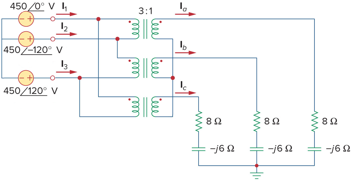
Figure 13.135 corrected, for Problem 13.73
In addition there are errata in this problem's answers given at the back of the textbook.
(Posted 4/26/2017, updated 4/19/2018)
Page 640. Example 14.11, final answer
The unit on the final answer should be μF, not πF.
Change the answer from "2.653 πF" to "2.653 μF.".
(Posted 11/05/2018, courtesy of e-mail from B. Dowling)
Page A-23. Answer to Problem 4.9
The wrong answer is printed. Correct it as follows:
(Posted 1/26/2017.)
Page A-25. Answer to Problem 5.39
The wrong answer is printed. Correct it as follows:
(Posted 2/09/2017.)
Page A-27. Answer to Problem 6.67.
Change "100cos(50t) mV" to
"100[cos(50t) – 1] mV"
(Posted 2/14/2017)
Page A-28. Answer to Problem 7.15.
The answer for the Thevenin equivalent resistance in part (b) is wrong.
(a) 10 Ω, 500 ms, (b)
(Posted 3/01/2017)
Page A-29. Answer to Problem 7.31(a).
The answer to part (a) is poorly rounded and in non-standard notation.
The correct answer to five places is 1.1254 × 10⁻⁷. Rounding gives. . .
(Posted 3/09/2018)
Page A-32. Answer to Problem 9.1(d).
Delete "0.3 rad"
(d) 44.48 V
(Posted 3/09/2017)
Page A-32. Answer to Problem 9.23(a).
The unit should be "V", not "A".
(a) 320.1 cos(20t - 80.11°) V
(Posted 3/21/2017)
Page A-32. Answers to Problem 11.47.
The negative signs in the answer to part (b) should both be positive. In part (c) the letter "k" for "kilo" is missing in two places. In all four parts, the variable S should be boldface since it is a complex amount in general. The text could be formatted more nicely for parts (c) and (d). A corrected version of the answer is shown below.
(a) S = (339.4 + j339.4) VA,
average power = 339.4 W,
reactive power = 339.4 VAR
(b) S = (678.8 + j678.8) VA,
average power = 678.8 W
reactive power = 678.8 VAR
(c) S = (7.637 + j7.637) kVA,
average power = 7.637 kW
reactive power = 7.637 kVAR
(d) S = (250 + j433) kVA,
average power = 250 kW
reactive power = 433 kVAR
(Posted 4/07/2017)
Page A-35. Answer to Problem 11.63(a).
The sign of the angle is wrong in the textbook
123.9/ –18.43° A rms.
(Posted 4/07/2017)
Page A-35. Answer to Problem 12.21(a).
The sign of the –60° angle is wrong in the textbook
44.00/ –30.00° A rms,
(Posted 4/19/2017)
Page A-36. Answer to Problem 12.71 part (b).
The answer for part (b) is wrong. The correct answer is. . .
(b)
Since the load is unbalanced the formula Q = √3(P2 – P1) does not apply.
See also the errata for page 535 and the alternative development of Equation 12.67.
(Posted 1/28/2017)
Page A-37. Answer to Problem 13.67(b).
The answer to part (b) is wrong. The load current is shown as the answer, but the secondary current is what was asked for. Also, although rms units can be assumed in this context, it would be better to explicitly mention them. The correct answers are:
(a) 352 V rms, (b)
(Posted 4/21/2017)
Page A-37. Answer to Problem 13.73 (b and c).
The answers printed for parts (b) and (c) are wrong.
(b)
I2 = 15.00/–83.13° A, Ic = 25.98/–173.13° A
(c)
16.20 kW
Also see the errata for the problem statement.
(Posted 4/26/2017, updated 5/01/2017)
Extensions and Clarifications of text material (Not errata.)
Page 457. More information on Eq. (11.5).
Equation (11.5) can be further developed to show the reactive power component. As with the development of Equation 11.5 in the textbook, this discussion and the related definitions below assume the voltage and current are sinusoidal.
Rearranging the second term in Eq. (11.5) to deliberately itemize the angle (θv – θi), the same as in the first term, gives
p(t) = (1/2)VmIm cos(θv – θi) + (1/2)VmIm cos[(2ωt + 2θv) – (θv – θi)]
Now apply the trigonometric identity cos(α – β) = cos(α)cos(β) + sin(α)sin(β)
to the second term to get
p(t) = (1/2)VmIm cos(θv – θi) +
(1/2)VmIm cos(2ωt + 2θv)cos(θv – θi) +
(1/2)VmIm sin(2ωt + 2θv)sin(θv – θi)
Associate the middle term above with the first term and factor out amounts that are constant with respect to time. The instantaneous power then is:
p(t) = (1/2)VmIm cos(θv – θi)[1 + cos(2ωt + 2θv)] +
(1/2)VmIm sin(θv – θi)sin(2ωt + 2θv)] (11.5b)
The first term above in Eq. (11.5b) pulsates due to the multiplicative term
[1 + cos(2ωt + 2θv)]. This multiplicative term has a maximum of 2, a minimum of 0, and an average of 1. Importantly, it is never negative. This means that the power represented by the first term always represents the rate of actual work. (Whether the work is absorbed or generated depends on the angle θv – θi and the sign convention associated with the labels that define the polarities of Vm and Im.) Since the average of the multiplicative term is 1, the coefficients on this multiplicative term represent the average power, P. This represents the average rate of actual work.
P = (1/2)VmIm cos(θv – θi)
The above equation is identical to Eq. (11.8) on page 458 in the text.
Turning our attention to the second term in Eq. (11.5b) notice that it's pulsation is represented by the multiplicative term, sin(2ωt + 2θv) This multiplicative term varies both positive and negative as time varies. This term has an average value of zero. It represents power that is surging back and forth as the algebraic sign of sin(2ωt + 2θv) oscillates. Thus this power does no useful work. This second term in Eq. (11.5b) is called the instantaneous reactive power. Although at any instant there is an amount of power flow related to this term, there is actually an amount of energy that surges back and forth with each cycle of the alternating current. The peak magnitude of the instantaneous reactive power is proportional to the amount of energy that oscillates back and forth. Thus the amount of reactive power is defined as the peak of the instantaneous reactive power. We use the variable Q to represent reactive power. Reactive power is given the units of "volt-amperes reactive" and is abbreviated as "VAR" or "VARs" (plural). This abbreviation is often pronounced as a word. The peak magnitude of the second term in Eq (11.5b) is
Q = (1/2)VmIm sin(θv – θi)
DEFINITION: Reactive power is the peak magnitude of power that surges equally back and forth. It has units of volt-amperes reactive (VAR).
(This definition and the related discussion here are valid for single-phase systems with sinusoidal voltages and currents. Otherwise this issue is more complicated.)
Now the instantaneous power, Eq. (11.5b), can be expressed in terms of the average power, P, and the reactive power, Q.
p(t) = P[1 + cos(2ωt + 2θv)] + Qsin(2ωt + 2θv) (11.5c)
In Section 11.4 of this textbook it is shown that
Vrms = Vm/√2 and that Irms = Im/√2
Applying these equalities gives.
P = VrmsIrms cos(θv – θi) , Q = VrmsIrms sin(θv – θi)
The above equations match Eq. (11.50) on page 472 of the text.
This illustrates the calculation of the average power and the reactive power for sinusoidal currents and voltages. The angle (θv – θi) recurs many times in discussions of AC circuits. For this reason in most textbooks and magazine articles it is simply denoted as θ. This angle is given the name power factor angle.
DEFINITION: The power factor angle or more simply, the power angle is
by definition θ = (θv – θi).
(This definition and the related discussion here are valid for single-phase systems with sinusoidal voltages and currents. With care to use phase voltages and currents or line voltages and currents and to not mix these, this definition may also be used with balanced three-phase systems that have sinusoidal voltages and currents.)
Using this definition, Eq. 11.50 on page 472 can be reduced to
P = VrmsIrms cos(θ) , Q = VrmsIrms sin(θ)
(Posted 3/19/2012)
Page 469. Eq 11.38a.
This equation subtly introduces phasors with RMS magnitudes.
In the power systems industry phasors are stated with RMS magnitudes rather than peak magnitudes. There are more implications to this than first meets the eye. In particular, the phasor transform is modified so that the phasor magnitude is in RMS units. Up to this point in this textbook, all phasor magnitudes have been peak magnitudes. In electronics work, peak magnitudes are usually used, but in power systems work RMS magnitudes are usually used.
Consider this electronics-style phasor transform having peak magnitude. This is the way the phasor transform has been used for everything in this book up to this point.
v(t) = 14.14cos(ωt + 25°) V <—> V = 14.14/25° V
Now the very same function in a power systems-style phasor transform will have an RMS magnitude. This type of phasor transform is used for everything from this point through the end of Chapter 12.
v(t) = 14.14cos(ωt + 25°) V <—> Vrms = 10/25° VRMS
Just like it is fair to say that 1 foot = 12 inches, it is also fair to say that
14.14/25° V = 10/25° VRMS because of the different units employed. And of course, the inverse transform of either style phasor is v(t) = 14.14cos(ωt + 25°) V.
However in this textbook, and in the general literature on power systems, the "RMS" subscript on the variable Vrms and on the unit "volts RMS" is usually omitted. The reader should understand that "unless otherwise stated" the units are RMS units when the context is power systems. For example consider Equation 11.41 on page 471. The equation is S = VrmsI*rms. The very same equation appears again in Equation 11.55 on page 476, but now the subscripts are missing, S = VI*. It means exactly the same thing and the magnitudes of the voltage and current phasors are still intended to be in RMS units, even though the subscripts are missing, because it occurs in the context of a chapter on electrical power (not a chapter on radio circuits for example).
(Posted 1/28/2017.)
Page 510–511 in reference to Figure 12.14.
The phrases "line voltage," "line-to-line voltage," "line-to-neutral voltage," "phase voltage," and similar terms for current such as, "phase current," can become confusing. Figure 12.14 can help us understand these. (The Internet is often unhelpful on the definitions of these terms since there are many such definitions of dubious authority posted on the Internet!) Here is a glossary of these terms with reference to Figure 12.14 on page 510.
Voltage, line voltage, line-to-line voltageReferences:
In the context of a three phase circuit whenever "voltage" is mentioned with no other description it should be assumed to be line-to-line voltage. Also, "line voltage" means "line-to-line voltage." In Figure 12.14 Vab is a line voltage. Other line voltages are Vbc and Vca.
Line-to-neutral voltage
Just as the name says, any line to neutral. Examples of line-to-neutral voltages In Figure 14.10 are, Van, Vbn and Vcn.
Phase voltage
The word "phase" refers to a physical 1/3 of a source or load. A phase voltage is the voltage across a 1/3 section of a source or load. In order to understand if this is a line-to-line voltage or a line-to-neutral voltage one needs to know if the source or load in the present context is Y or Δ connected. In Figure 12.14, Van is a phase voltage for the source and Vbc is a phase voltage for the load. (There are many confusing definitions of "phase voltage" on the Internet. In many cases these definitions happen to be in the context of a Y connection and they state only that phase voltage is a line-to-neutral voltage. They fail to mention that in the context of a Δ connection phase voltage is line-to-line voltage. The explanation is correct in its Y-connected context on the Web, but is incomplete for general use.)
Line current
Self explanatory. In Figure 12.14 Ia, Ib, and Ic are the line currents.
Phase current
The word "phase" refers to a physical 1/3 of a source or load. A phase current is the current through a 1/3 section of a source or load. In order to understand if this is a line current or something else one needs to know if the source or load in the present context is Y or Δ connected. In Figure 12.14, Ia is a phase current for the source and IAB is a phase current for the load. (There are many confusing definitions of "phase current" on the Internet. In many cases these definitions happen to be in the context of a Y connection and they state only that phase current is a line current. They fail to mention that in the context of a Δ connection phase current is something else. The explanation is correct in its Y-connected context on the Web, but is incomplete for general use.)
Hadi Saadat, Power System Analysis, McGraw Hill. (various editions), See how the above phrases are used in Chapter 2
Ned Mohan, Electric Power Systems: A First Course Wiley, 2012. See the vocabulary in Chapter 2.
(Posted 4/21/2017)
Page 534–535 First paragraph in Sec. 12.10.
The first paragraph in Section 12.10 of the textbook contains some errors of substance and some poor grammar. Several paragraphs of replacement text are offered here. This replacement corrects the errors and offers a more complete explanation of the several issues the textbook's paragraph touches on.
In modern practice, the balanced wye connection is preferred for most three-phase sources. This is due to at least two factors. First, a balanced wye connection creates a neutral (center of the wye) that can be connected to earth for safety. Providing the source with this safety connection simplifies the design of other protection such as fusing. (Providing a neutral for a delta-connected source is a much more complicated matter. See for example here and here and here.) Secondly, single-phase loads can be most easily connected to a three-phase system by connecting them between any single line and neutral, but a delta connection does not provide a simple-to-use neutral for this purpose. For this reason three-phase 208 VRMS line-to-line systems are popular in North American commercial buildings. Then 120 VRMS single-phase loads are connected from line to neutral (208/√3 = 120). Similarly in Europe and some other geographic locations a 400 VRMS line-to-line three-phase power system is used to provide 230 VRMS from any one line to neutral. Delta connected sources are rarely specified for modern installations because any slight imbalance between the three phases can cause problematic circulating currents, and also because protection devices (e.g. fuses) are more complicated to use and maintain effectively.(Posted 3/19/2012.)
Circulating currents are not a problem in delta-connected loads however, because each phase has appreciable impedance so that it may absorb electrical power. Delta connected loads also operate at the full line-to-line voltage which is √3 greater than the line-to-neutral voltage. This can economically reduce heating (I2R) losses in some practical situations. If for some reason a delta-connected load is slightly electrically unbalanced (say one phase draws a bit more current than the others), connecting it to a wye source distributes the unbalance over two phases, making the system as a whole more balanced. For these practical reasons delta connections are popular for loads. However, in theory it is immaterial if a load is wye or delta connected.
For example, either a wye or a delta connection is satisfactory with induction motors. Some induction motors have terminal boards with six terminals, one for each end of the three windings. Then the customer can choose a wye or delta connection. In this way a manufacturer can offer one line of motors to operate at two different voltages. The higher rated voltage option will then be √3 greater than the lower rated option. For example a motor might be rated for 277 delta/480 wye VRMS. In this example the motor phases (coils) are designed to operate at 277 VRMS. The motor may be connected to a 277 VRMS line-to-line voltage system using a delta connection which gives each phase (coil) 277 VRMS. Alternatively, the same motor may be connected to a 480 VRMS line-to-line voltage system by using a wye connection. Then each phase (coil) will again be driven with 277 VRMS. Some of these motors are designed to start with the wye connection and then, as the motor comes up to speed, a set of relays switches it to the delta connection to bring it to full power for normal running conditions. Connecting the example motor above for wye-start-delta-run would require a 277 VRMS line-to-line three-phase power source. This starting method minimizes voltage brown-outs in the power supply system when the motor starts by minimizing the surge current needed to start the motor.
Other motors achieve a dual voltage rating by using dual windings for each of the three phases (six windings in total). These motors have terminal boards with nine terminals. The dual windings of each phase may then be connected in either series or parallel. Some connections are made inside the motor by the manufacturer and are not accessible to the user. These internal connections will make the motor connections either wye or delta as prescribed by the manufacturer. The customer will only have the choice of operating voltage, not wye or delta connection. The two voltage ratings will differ by a factor of two, for example 240/480 VRMS. The dual rating can also be used on a power system corresponding to the lower voltage rating to minimize the surge current needed to start the motor. In this case the motor is stared with the pairs of windings connected in series. Then, as the motor comes up to speed, a set of relays reconnects the windings in parallel for normal running. This type of starting method generally provides more starting torque than the wye-start-delta-run method.
Finally, some motors have dual windings and twelve terminals. These allow the customer up to four different operating voltages by choosing combinations of series and parallel windings and wye or delta connections. This flexibility may also be used to achieve a wye-start delta-run configuration at either of two voltage levels or a series-start-parallel-run configuration, again at either of two voltages.References:
EASA Engineering Handbook, "Three-Phase Motors—Single
Speed."
Hamid A. Toliyat, Gerald B. Kliman, editors, Handbook of Electric Motors
2nd edition revised and expanded, Marcel Dekker, Inc., 2004,
pages 455-456.
Roland E. Thomas, Albert J. Rosa, The Analysis and Design
of Linear Circuits, pp. 811–812, Prentice Hall, 1994.
Richard C. Dorf, James A. Svoboda, Introduction to Electric
Circuits, 8th Ed., p. 571, Wiley, 2010.
Hadi Saadat, Power Systems Analysis 2nd ed., page 31,
McGraw-Hill, 2002.
IEEE Recommended Practice for Electric Power Distribution
for Industrial Plants, 2nd ed., pp. 437-440, IEEE, New
York, 1986.
IEEE Recommended Practice for Electric Power Systems in
Commercial Buildings , pp. 127-130, IEEE, New York, 1983.
E. Lakervi, E.J. Holmes, Electricity Distribution Network
Design, pp. 110–112, Peter Peregrinus Ltd., London, 1989.
Eng-tips discussion forums, "advantages and disadvantages. . ."
Wikipedia, "Three-phase electric power."
Wikipedia, "Mains Electricity."
Page 534 Alternative development of Equation 12.67.
The textbook's development of Equation 12.67 is unnecessarily restricted to balanced loads. In Figure 12.35 one may take the load to be unbalanced. Identify each phase with a different load such as ZYa, ZYb, ZYc and assume that these are not necessarily equal to each other. Also consider node b (the phase b line) to be the ground reference. Now there are effectively only two voltage sources driving the load, Vab and Vcb as labeled in Figure 12.35. Each wattmeter measures the power supplied by one source. Thus it is self-evident that PT = P1 + P2, even if the load is unbalanced.
See also the errata for page 535 and the answer to Problem 12.71.
(posted 1/28/2017.)
Page 580 Example 13.10.
Although an autotransformer is customarily thought of as a transformer that employs one tapped winding as both the primary and the secondary, it is not necessarily constructed this way.
It can be helpful to think of an autotransformer as an ordinary transformer that is used in a special type of connection, the "autotransformer connection." Any transformer can be connected in an autotransformer connection, assuming it has adequate insulation which is usually the case. Below, Figure 13.43 has been augmented with part (c) to show how the transformer of part (a) can be connected to perform identically to the autotransformer of part (b).
When the voltage will be autotransformed by a small amount, that is by a ratio that is close to 1:1, then the turns ratio of the basic transformer, as in part (a) of Figure 13.43, needs to be far from 1:1. In this example the voltage transformation ratio is 20:21 and the turns ratio is 20:1. Then usually the winding with fewer turns needs to be made of larger gauge wire in order to carry the correspondingly larger current. Thus for the maximum economic benefit, the autotransformer illustrated in part (b) of the figure might actually be constructed from two windings connected as in part (c). This way the primary winding can be made from a thinner conductor since it does not need to carry the full 4 A load current. The transformer is still called an "autotransformer," as if it had only one winding, because of the presence of the connection that places the two physical windings into one electrical winding with a tap.
However, if the voltage transformation ratio is 1:2 then the turns ratio of the transformer is 1:1. This case is interesting because the current in each winding is identical in magnitude. For example if the turns ratio of the transformer in part (a) of the figure is changed to 1:1 then the secondary voltage changes to 240 V and the secondary current changes to 0.2 A. The transformer would be operating at
(240 V)(0.2 A) = 48 VA. But, in the autotransformer connection of part (c) the current flowing into the circuit from the left would be 0.4 A. This current would divide with 0.2 A going into the primary winding and 0.2 A going into the lower terminal of the secondary winding. Each winding experiences 0.2 A in this case. The net power delivered to the load would be 480 V at 0.2 A or 96 VA, which is two times greater than the transformer can handle when connected as a transformer. This is the type of situation in which a true single winding with a tap, as implied in the definition of an autotransformer, is economic in terms of a savings of copper and iron, and weight and size.
Regardless of the internal construction of an autotransformer (as truly one winding with a tap or as two physical windings of different gauge conductors connected in series) the economic advantages of an autotransformer are best realized when the voltage transformation ratio is between 2:1 and 1:2. When a wider voltage transformation ratio is needed, at some point the advantage of isolation that a standard transformer connection has becomes compelling and the economic advantage of the autotransformer dwindles in comparison.
See also the errata on this figure as published in the textbook.
(Posted 3/19/2012)
Disclaimer: This list of errata is provided by Professor De Boer for the use of his students in his courses. This list is offered as is, with no guarantee of any kind. (This list is likely to be incomplete at the least.)
Back to Prof. De Boer's home page