Professor De Boer's list of
TEXTBOOK ERRATA
(last update 1/05/2017)
Alexander & Sadiku,
Fundamentals of Electric Circuits, 5th Ed.
ISBN 978-0-07-338057-5, McGraw-Hill, 2012.
(link to errata for the 4th edition.
The errata for the 4th edition gets updated more frequently.
Since the 4th and 5th editions are almost page-for-page identical,
there could be more useful up-to-date information in the errata for the 4th edition.
Here is a link to errata for the 6th edition.
The sixth edition has corrected a lot of errata that has persisted through many previous editions.)
If you are considering purchasing this textbook and worrying that it is a poor choice due to the length of this list of errata, please don't worry about that. Competing textbooks have about as many errata, but perhaps no list like this. "Better the devil you know than the devil you don't." Professor De Boer likes this book enough to find it worthwhile to publish this list of errata.
First of all, check the author's official list of errata.Secondly, check Professor Reeder's list of errata for this textbook.
The following additional errata have been found to date:
When specific corrections are illustrated, additions are in blue text.
Deletions are instrikeout blue text. Commentary is in green text.
Page 5, The paragraph that starts, "As electrical. . ."
Replace "principal" with "base," improve the grammar, and identify the derived unit by changing the paragraph as follows:
As electrical engineers, we must deal with measurable quantities. Our mea-
surements, however, must be communicated in a standard language that
virtually all professionals can understand, irrespective of the country
where the measurement is conducted. Such an international measurement
language is the International System of Units (SI), adopted by the
General Conference on Weights and Measures in 1960. In this system,
there are seven
ical quantities can be derived. Table 1.1 shows
derived unit (the coulomb) that are related to this text.
"Principal" is the wrong word here. "Principle" was intended by the authors but the standards actually use the word "base." Also as it stands in the text, the poor grammar makes the number of base units ambiguous as either six or seven. Finally, "The SI units. . ." is a weak way to state the intention of this sentence. Most students would not comprehend the intent. (The SI base unit not mentioned in Table 1.1 is the mole.) For reference see:Page 7, The highlighted text boxes and nearby text on the lower third of the page.
Bureau International des Poids et Mesures
National Institute of Standards and Technology
(Posted 3/19/2012.)
Both of these definitions are overly restrictive. Additionally, the text around them conflates the concept of a constant current versus a time-varying current with the concepts of dc versus ac. Correct the surrounding text and the definitions, starting with the paragraph that begins with, "If the current does not change. . ."
If the current does not change with time,
Current can also be classified as direct or alternating.
A direct current (dc) is a current that never reverses direction.
Direct current could be time-varying. For example, i(t) = –|3cos(377t)| A
is a direct current because it never changes sign, indicating that it never reverses
direction.
A time-varying curer is represented by the symbol i. A common
form of time-varying current is the sinusoidal current or alternating current (ac).
An alternating current (ac) is a current that changes direction from time to time.
Such current is used in your household, to run the air conditioner,
refrigerator, washing machine, and other electric appliances. Figure 1.4
There are various definitions of dc and ac in the literature. The definitions created by these corrections represent the more commonly found definitions. A statement such as, "A rectifier converts ac to dc." is consistent with the definitions given by the corrections above, but not the uncorrected definitions in the textbook. (The "dc" current that flows out of a rectifier is usually not constant with respect to time. The waveform of the "ac" current that flows into a rectifier is usually not sinusoidal.) A direct current does not have to be a constant amount. It may pulsate or otherwise vary with time so long as it does not reverse direction.Page 9, The line above Eq. 1.3
It is philosophically satisfying that we should be able to classify a current as either dc or ac. The definitions in the textbook allow for currents that are neither dc or ac, for example, a triangle wave that oscillates between 1 A and –1 A. By allowing alternating current to have any waveform and any period or no period (aperiodic) so long as it changes direction from time to time, all currents can then be classified as dc or ac.
(Posted 10/06/2012, updated 10/09/2012)
a unit charge from
Voltage is measured between two specific points and it has a defined polarity. It is conventional that the second subscript in a voltage variable is the reference point. In Equation 1.3 the second subscript is b. Thus b is the reference point, or the the starting point where the charge is initially located. For reference see:Page 9, The the highlighted text box
Halladay, Resnik, and Walker, Fundamental of Physics, Part 3, 8e, John Wiley & Sons, Inc., 2008, see Chapter 24 and especially Equation 24-6.
(Posted 3/19/2012, explanation updated 3/30/2012.)
Voltage (or potential difference) is the energy required to move a unit
charge
Voltage is defined between two specific points (no circuit element is needed) and it has a defined polarity. For reference see:Page 23. Summary, point 4
Halladay, Resnik, and Walker, Fundamental of Physics, Part 3, 8e, John Wiley & Sons, Inc., 2008, see Chapter 24 and especially Equation 24-6.
(Posted 4/24/2012.)
4. Voltage is the energy required to move 1 C of charge
Also, in the equation that follows this sentence replace "v" with "vab."
Voltage is defined with respect to two points. The pathway, "through an element," is irrelevant. Any path from b to a results in the same voltage.Page 27. Problem 1.34 part (b)
See also the comment for the errata on page 9.
(Posted 3/19/2012. updated 4/24/2012)
(b) the average power
period.
"Power per hour" is a the rate of change of power. It may be used to characterize the ramp rate of an electric power generating station, but it has nothing to do with this problem. Just plain "average power" is the authors' intent. Reference: "Confusion of watts, watt-hours, and watts per hour" section of the Wikipedia article "Watt" (Posted 3/19/2012.)Page 59. Figure 2.55 part (b)
Near the symbol for the plug an extranious line (creating a short circuit) needs to be removed. A corrected illustration is shown below.
Figure 2.55 (b) Corrected.
(Posted 4/06/2012.)
Page 60. Practice Problem 2.16
Change the problem statement to read as follows:
Refer to Fig. 2.55 and assume there are 10 light bulbs that can be con-
nected in parallel and 10 different light bulbs that can be connected in series
In either case, each light bulb is to operate at
If the voltage at the plug is 110 V for the parallel and series connections,
calculate the current through and the voltage accress each bulb for both cases.
Answer: 364 mA, 110 V (parallel); 3.64 A, 11.0 V (series)
As written, the problem is ambiguous. Most students assume the situation of a familiar high-school physics experiment in which a few light bulbs are connected in parallel and then the same light bulbs are reconnected in series. This is not the author's intent for this practice problem.Page 75. Problem 2.61, the last line
(Posted 4/06/2012.)
An "I" is missing. Change the last line of the problem statement to read as follows:
such that I lies within the range I = 1.2 A ±5 percent.
(Posted 1/05/2017.)
Page 119. Problem 3.34
As printed, what is being requested is not precisely clear, especially for students who are learning the concept of a planar circuit. Change the problem statement so that it reads as follows:
For each
If it is planar
(Posted 1/05/2017.)
Page 164. Problem 4.20
Replace the problem with the following:
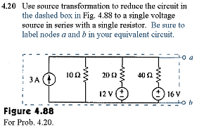
Without the changes shown there is no reasonable way to apply the concept of equivalency in order to reduce the circuit in a meaningful way. The changes to the figure are the addition of the dashed box, and the addition of the terminals labeled "a" and "b."Page 221. Equations near the top of the page.
(posted 3/19/2012)
*Change the variable of integration from t to λ. Do not change the limit. This is the first of a number of similar errors in this textbook. See the note marked by an asterisk below on this page. In this case, the correct equations (with minimal editing) are:
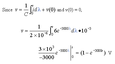
Or with more extensive editing to completely show the various functional dependencies:
(Posted 3/19/2012.)
Page 249. Problem 6.67.
An initial condidtion is needed to solve this problem. Add it to the end of the problem statement. The problem is then as follows:
6.67 An op amp integrator has R = 50 kΩ and C =
0.04 μF. If the input voltage is vi = 10sin50t mV,
optain the output voltage. Assume that at t = 0
the output voltage is zero.
(Posted 9/26/2012.)
Page 321. Five lines below Equation 8.11
second (rad/s); and α is the neper frequency
Also see related errata on pages 323, 361, and I-2.
The phrase, neper frequency is preferable for naming the quantity denoted by α in this textbook. In addition to the definition of damping factor implied in this textbook, the phrase damping factor has a plurality of other definitions applying in other contexts. For three unique examples see here and here (in "Variations and hybrid methods" section) and this textbook (See page 506 of the textbook). Furthermore, Prof. De Boer has not so far found any place where the phrase damping factor is treated synonymously with neper frequency except in undergraduate circuits and linear systems textbooks or World Wide Web pages intended for that same audience. This limited context is too narrow to justify introducing the phrase damping factor here.Page 323. The lines below Equation 8.22b
A nearly similar term, damping ratio, (not "factor") is uniformly well defined in many contexts, including RLC circuits, but the neper frequency (α in our textbook) and the damping ratio are not the same thing. Usually the damping ratio is represented by the variable ζ (zeta). Using our textbook's notation, the damping ratio would be defined as ζ = α/ωo. Since most engineering students will encounter the term damping ratio in their careers, the confusingly similar name, damping factor (also known as damping attenuation factor, attenuation factor, and damping coefficient, etc.) should not be introduced in the context of RLC circuits. The name neper frequency for α is more memorable, more universal in the literature, and thus more helpful.
(Posted 3/19/2012)
and also about ten lines from the bottom of the page
On the line below Equation 8.22b change the phrase,
"damping frequency" to "damped frequency"
where j = √ –1 and ωd = √ ωo2 – α2, which is called the damped
Also, about ten lines from the bottom of the page, change
"The damping factor. . ." to "The neper frequency. . ."
. . .due to the presence of resistance R. The
α determines the rate at which. . .
Also see related errata on pages 321, 361, and I-2.
The name "damping frequency" is incorrect—a grammatic error. "Damped frequency" is one of several names commonly used for this quantity.Page 361. Problem 8.23References:(Posted 3/19/2012)
Katsuhiko Ogata, Modern Control Engineering, fifth edition,
Prentice Hall, 2010, page 166.
Norman S. Nise, Control Systems Engineering, fourth edition,
Wiley, 2004, page 197.
Richard C. Dorf, Modern Control Engineering, twelfth edition,
Prentice Hall, 2011, Page 567.
James W. Nielson, Electric Circuits, fourth edition,
Addison Wesley, 1994, page 332.
Wikipedia article on "Damping"
Change "damping factor" to "neper frequency."
Also see related errata on pages 321, 323, and I-2.
(Posted 3/19/2012.)
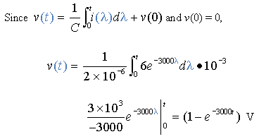
Page 363. Problem 8.45, Figure 8.92
The Figure is inconsistent with the given assumptions. In particular, i(0) would be zero based on Figure 8.45 as it is printed. To correct this error, add a 1 A source as shown below and change "4u(t) A" to "3u(t) A."
(An interesting variation on the above problem is to change the value of R from 2 Ω to 1 Ω. In this case, the answers are v(t) = 6e-tsin(t) V andPage 405. Problem 9.29
i(t) = 4 – 3e-t[cos(t) + sin(t)] A
(Posted 3/19/2012, updated 10/26/2012)
Add, "Given that v(0) = 2cos(155°) V" to the beginning of the problem statement. The problem statement then reads as follows:
9.29 Given that v(0) = 2cos(155°) V,
instantaneous voltage across a 2-μF capacitor
when the current through it is
i = 4sin(106t + 25°) A?
(Posted 3/19/2012.)
Page 405. Problem 9.35
Add "the steady-state" between the word "Find" and "current."
The problem then reads:
9.35 Find the steady-state current i in . . .
(Posted 3/19/2012.)
Page 495. Problem 11.48
Two minus signs are missing.
In part (a) change "Q = 150 VAR," to "Q = –150 VAR."
In part (b) change "Q = 2000 VAR," to "Q = –2000 VAR."
Also, the words "capacitive" and "inductive" should be deleted from parts (a) and (c). The problem then reads as:
11.48 Determine the complex power for the following
cases:
(a) P = 269 W, Q = –150 VAR
(b) Q = –2000 VAR, pf = 0.9 (leading)
(c) S = 600 VA, Q = 450 VAR
(d) Vrms = 220 V, P = 1 kW
| Z | = 40 Ω (inductive)
The words "capacitive" and "inductive" can be applied to an impedance, especially an impedance magnitude as in part (d). They can also be applied to the power factor in lieu of "leading" and "lagging" respectively, but these words are not correct with respect to reactive power. "Capacitive" reactive power is always negative. Similarly, "Inductive" reactive power is always positive. Stating a positive reactive power and calling it "capacitive" is confusingly incorrect. Similarly, the terms "leading" and "lagging" should not be used with respect to a quantified (numerically) reactive power either in lieu of or to augment an algebraic sign. ("Capacitively generated reactive power" is a meaningful statement however. The word "Capacitively" does not modify "reactive power" in this case.)Page 506. Figure 12.5
(Posted 3/19/2012, explanation updated 3/30/2012)
The labels at the top of the figure, Van(t), Vbn(t), and Vcn(t) should be replaced by van(t), vbn(t), and vcn(t) respectively.
This is a time-domain figure. Capital letters indicate phasors. This is incongruent with the domain of the figure and the notation elsewhere in this textbook. (Posted 3/19/2012)Pages 534–535 First paragraph in Sec. 12.10.
This paragraph contains poor grammar and some substantive errors. It also touches on some complicated issues. For a more complete discussion of this paragraph see the entry in the "Extensions and Clarifications" section of this document. Only corrections are shown here.
Both the wye and delta connections have important practical appl-
ications. The wye source connection is used for long distance trans-
mission of electric power, where resistive losses (I2R) should be
______(page break)_______
voltage that is √3 greater than the delta connection, hence for the same
power, the line current is √3 smaller.
rents.
connect source.
This conversion from three-phase to single phase is required in
because
ances use single-phase power. Three-phase power is used
wiring
terial whether the load is wye- or delta-connected. For example, both
connections are satisfactory with induction motors.
ufacturers connect a motor in delta for 220 V and in wye for 440 V so
that one line of motors can be readily adapted to two different voltages.
References:Page 544. Problem 12.7
Roland E. Thomas, Albert J. Rosa, The Analysis and Design
of Linear Circuits, pp. 811–812, Prentice Hall, 1994.
Richard C. Dorf, James A. Svoboda, Introduction to Electric
Circuits, 8th Ed., p. 571, Wiley, 2010.
Hadi Saadat, Power Systems Analysis 2nd ed., page 31,
McGraw-Hill, 2002.
IEEE Recommended Practice for Electric Power Distribution
for Industrial Plants, 2nd ed., pp. 437-440, IEEE, New
York, 1986.
IEEE Recommended Practice for Electric Power Systems in
Commercial Buildings , pp. 127-130, IEEE, New York, 1983.
E. Lakervi, E.J. Holmes, Electricity Distribution Network
Design, pp. 110–112, Peter Peregrinus Ltd., London, 1989.
Eng-tips discussion forums, "advantages and disadvantages. . ."
Wikipedia, "Three-phase electric power."
(Posted 3/19/2012. updated 3/30/2012)
The word "phasor" is missing.
Obtain the phasor line currents in the. . .
If a "phasor" amount is not specifically requested then by convention the answer should correspond to that which a VOM or DMM would read, which is only the magnitude the phasor amount. In this case the complete phasor amount is the desired answer, thus it should be specifically requested.Page 548. Problem 12.36(c)
(Posted 3/19/2012.)
Insert the phrase "line-to-neutral."
(c) the line-to-neutral voltage at the sending end.
In three-phase systems it is conventional to assume line-to-line voltage is if nothing is specified.Page 551. Problem 12.66
(Posted 3/19/2012.)
More information needs to be given in order to get the author's intended answers. Change the problem statement to read as below:
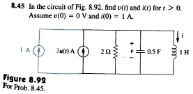
12.66 A three-phase, four-wire system operating with aPage 582 Figure 13.43 and Example 13.10.
208-V line voltage is shown in Figure 12.71. The
source voltages are balanced. The voltage of phase 1
is the reference phasor. The phase sequence is 1, 2, 3.
The power absorbed by the resistive wye-connected
load is measured by the three-wattmeter method.
Calculate:
(a) the line-to-neutral voltageto neutral
(b) the currents I1, I2, I3, and In,
(c) the readings of the wattmeters
(d) the total power absorbed by the load
(Posted 3/19/2012.)
Add dots near the top of each coil (four instances) to show flux polarity. (Voltage labels do not indicate flux polarity. They indicate voltage!) A corrected illustration is shown below.
In an autotransformer connection correct flux linkage depends importantly on flux polarities. The illustrations need to have dots added to the transformer windings to show flux polarities even though in this case all the "+" marks coincidentally correspond to places where a dot is needed. See also the elaboration of this figure in the "Extensions and Clarifications" section below.
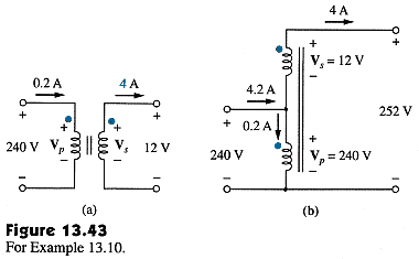
(Posted 3/19/2012, updated 8/29/2012)
Page 636 Example 14.8
In figure 14.27 change the 10 sin(ωt) V voltage source to a 1.25 sin(ωt) mA current source.
In part (c) of the solution, delete "Y = 1/R or" and delete the entire equation that starts, "Io ="
If the circuit is driven with a voltage source the power dissipation will not be frequency dependent. To support Example 14.8, the parallel RLC circuit must be driven by a current source. (By duality, a series RLC circuit would have to be driven by a voltage source if the power dissipation is to be frequency dependent.)
(Posted 3/20/2015.)
Page I-2. About 13 lines from the bottom of the second column
Delete the index entry for "Damping factor."
Change the index entry for "Damping frequency" to "damped frequency."
Also see related errata on pages 321, 323, and 361.
(Posted 3/19/2012.)
*This textbook contains a systematic error.
In some cases where an expression is integrated with respect to time the same variable, t, is used as the variable of integration and as the upper limit of the integral. One variable should not be used for two different quantities. In these cases some other variable such as λ should be substituted for the variable of integration. As an example, the first instance of this error is in the equations near the top of page 221. Some other instances of this error include:
Equations on pages, 229, (three instances), 231 (seven instances), 233, (four instances), 241 (four instances), 250 (two instances)
Some other instances of this problem likely have not yet been itemized in this errata sheet. Furthermore, in many cases where this situation arises and it is correctly handled, the authors have used the variable τ as the variable of integration. This invites confusion with the quantity known as a time constant, also represented by τ. Readers need to understand that two different quantities (variable of integration or time constant) are denoted by τ in this textbook. The meaning of τ must be discerned by the reader from its context.
(Posted 3/19/2012)
Extensions and Clarifications of text material (Not errata.)
Page 459. More information on Eq. (11.5).
Equation (11.5) can be further developed to show the reactive power component. As with the development of Equation 11.5 in the textbook, this discussion and the related definitions below assume the voltage and current are sinusoidal.
Rearranging the second term in Eq. (11.5) to deliberately itemize the angle (θv – θi), the same as in the first term, gives
p(t) = (1/2)VmIm cos(θv – θi) + (1/2)VmIm cos[(2ωt + 2θv) – (θv – θi)]
Now apply the trigonometric identity cos(α – β) = cos(α)cos(β) + sin(α)sin(β)
to the second term to get
p(t) = (1/2)VmIm cos(θv – θi) +
(1/2)VmIm cos(2ωt + 2θv)cos(θv – θi) +
(1/2)VmIm sin(2ωt + 2θv)sin(θv – θi)
Associate the middle term above with the first term and factor out amounts that are constant with respect to time. The instantaneous power then is:
p(t) = (1/2)VmIm cos(θv – θi)[1 + cos(2ωt + 2θv)] +
(1/2)VmIm sin(θv – θi)sin(2ωt + 2θv)] (11.5b)
The first term above in Eq. (11.5b) pulsates due to the multiplicative term
[1 + cos(2ωt + 2θv)]. This multiplicative term has a maximum of 2, a minimum of 0, and an average of 1. Importantly, it is never negative. This means that the power represented by the first term always represents the rate of actual work. (Whether the work is absorbed or generated depends on the angle θv – θi and the sign convention associated with the labels that define the polarities of Vm and Im.) Since the average of the multiplicative term is 1, the coefficients on this multiplicative term represent the average power, P. This represents the average rate of actual work.
P = (1/2)VmIm cos(θv – θi)
The above equation is identical to Eq. (11.8) on page 460 in the text.
Turning our attention to the second term in Eq. (11.5b) notice that it's pulsation is represented by the multiplicative term, sin(2ωt + 2θv) This multiplicative term varys both positive and negative as time varys. This term has an average value of zero. It represents power that is surging back and forth as the algebraic sign of sin(2ωt + 2θv) oscillates. Thus this power does no useful work. This second term in Eq. (11.5b) is called the instantaneous reactive power. Although at any instant there is an amount of power flow related to this term, there is actually an amount of energy that surges back and forth with each cycle of the alternating current. The peak magnitude of the instantaneous reactive power is proportional to the amount of energy that oscillates back and forth. Thus the amount of reactive power is defined as the peak of the instantaneous reactive power. We use the variable Q to represent reactive power. Reactive power is given the units of "volt-amperes reactive" and is abbreviated as "VAR" or "VARs" (plural). This abbreviation is often pronounced as a word. The peak magnitude of the second term in Eq (11.5b) is
Q = (1/2)VmIm sin(θv – θi)
DEFINITION: Reactive power is the peak magnitude of power that surges equally back and forth. It has units of volt-amperes reactive (VAR).
(This definition and the related discussion here are valid for single-phase systems with sinusoidal voltages and currents. Otherwise this issue is more complicated.)
Now the instantaneous power, Eq. (11.5b), can be expressed in terms of the average power, P, and the reactive power, Q.
p(t) = P[1 + cos(2ωt + 2θv)] + Qsin(2ωt + 2θv) (11.5c)
In Section 11.4 of this textbook it is shown that
Vrms = Vm/√2 and that Irms = Im/√2
Applying these equalities gives.
P = VrmsIrms cos(θv – θi) , Q = VrmsIrms sin(θv – θi)
The above equations match Eq. (11.50) on page 474 of the text.
This illustrates the calculation of the average power and the reactive power for sinusoidal currents and voltages. The angle (θv – θi) recurs many times in discussions of AC circuits. For this reason in most textbooks and magazine articles it is simply denoted as θ. This angle is given the name power factor angle.
DEFINITION: The power factor angle or more simply, the power angle is
by definition θ = (θv – θi).
(This definition and the related discussion here are valid for single-phase systems with sinusoidal voltages and currents. With care to use phase voltages and currents or line voltages and currents and to not mix these, this definition may also be used with balanced three-phase systems that have sinusoidal voltages and currents.)
Using this definition, Eq. 11.50 on page 474 can be reduced to
P = VrmsIrms cos(θ) , Q = VrmsIrms sin(θ)
(Posted 3/19/2012)
Page 471. Eq 11.38a.
This equation subtly introduces phasors with RMS magnitudes.
In the power systems industry phasors are stated with RMS magnitudes rather than peak magnitudes. There are more implications to this than first meets the eye. In particular, the phasor transform is modified so that the phasor magnitude is in RMS units. Up to this point in this textbook, all phasor magnitudes have been peak magnitudes. In electronics work, peak magnitudes are usually used, but in power systems work RMS magnitudes are usually used.
Consider this electronics-style phasor transform having peak magnitude. This is way the the phasor transform has been used for everything in this book up to this point.
v(t) = 14.14cos(ωt + 25°) V <—> V = 14.14/25° V
Now the very same function in a power systems-style phasor transform will have an RMS magnitude. This type of phasor transform is used for everything from this point through the end of Chapter 12.
v(t) = 14.14cos(ωt + 25°) V <—> Vrms = 10/25° VRMS
Just like it is fair to say that 1 foot = 12 inches, it is also fair to say that
14.14/25° V = 10/25° VRMS because of the different units employed. And of course, the inverse transform of either style phasor is v(t) = 14.14cos(ωt + 25°) V.
However in this textbook, and in the general literature on power systems, the "RMS" subscript on the variable Vrms and on the unit "volts RMS" is usually omitted. The reader should understand that "unless otherwise stated" the units are RMS units when the context is power systems. For example consider Equation 11.41 on page 473. The equation is S = VrmsI*rms. The very same equation appears again in Equation 11.55 on page 478, but now the subscripts are missing, S = VI*. It means exactly the same thing and the magnitudes of the voltage and current phasors are still intended to be in RMS units, even though the subscripts are missing, because it occurs in the context of a chapter on electrical power (not a chapter on radio circuits for example).
Note also in passing that boldface denotes a phasor (complex in general) and normal text denotes a real number and that Vrms = |Vrms|. Similarly, S = |S|.
(Posted 3/19/2012.)
Page 534–535 First paragraph in Sec. 12.10.
The first paragraph in Section 12.10 of the textbook contains some errors of substance and some poor grammar. Several paragraphs of replacement text are offered here. This replacement corrects the errors and offers a more complete explanation of the several issues the textbook's paragraph touches on.
In modern practice, the balanced wye connection is preferred for most sources. This is due to at least three factors. First, a balanced wye connection creates a neutral (center of the wye) that can be connected to earth for safety. Providing the source with this safety connection simplifies the design of other protection such as fusing. (Providing a neutral for a delta-connected source is a much more complicated matter. See for example here and here and here.) Secondly, single-phase loads can be most easily connected to a three-phase system by connecting them between any single line and neutral, but a delta connection does not provide a simple-to-use neutral for this purpose. For this reason three-phase 208 VRMS line-to-line systems are popular in North American commercial buildings. Then 120 VRMS single-phase loads are connected from line to neutral (208/√3 = 120). Similarly in Europe and some other geographic locations a 400 VRMS line-to-line three-phase power system is used to provide 230 VRMS from any one line to neutral. Thirdly, connecting a given set of windings in a three-phase source in a wye connection gives line voltages that are a factor of √3 greater than a delta connection would give. In the case of long distance power transmission, higher line voltages reduce the line currents and consequently reduce the power losses (I2R) caused by heating of the conductors. Delta connected sources are rarely specified for modern installations because any slight imbalance between the three phases can cause problematic circulating currents, and also because protection devices (e.g. fuses) are more complicated to use and maintain effectively.(Posted 3/19/2012.)
Circulating currents are not a problem in delta-connected loads however, because each phase has appreciable impedance so that it may absorb electrical power. Delta connected loads also operate at the full line-to-line voltage which is √3 greater than the line-to-neutral voltage. This can economically reduce heating (I2R) losses in some practical situations. If for some reason a delta-connected load is slightly electrically unbalanced (say one phase draws a bit more current than the others), connecting it to a wye source distributes the unbalance over two phases, making the system as a whole more balanced. For these practical reasons delta connections are popular for loads. However, in theory it is immaterial if a load is wye or delta connected.
For example, either a wye or a delta connection is satisfactory with induction motors. Some induction motors have terminal boards with six terminals, one for each end of the three windings. Then the customer can choose a wye or delta connection. In this way a manufacturer can offer one line of motors to operate at two different voltages. The higher rated voltage option will then be √3 greater than the lower rated option. For example a motor might be rated for 277 delta/480 wye VRMS. In this example the motor phases (coils) are designed to operate at 277 VRMS. The motor may be connected to a 277 VRMS line-to-line voltage system using a delta connection which gives each phase (coil) 277 VRMS. Alternatively, the same motor may be connected to a 480 VRMS line-to-line voltage system by using a wye connection. Then each phase (coil) will again be driven with 277 VRMS. Some of these motors are designed to start with the wye connection and then, as the motor comes up to speed, a set of relays switches it to the delta connection to bring it to full power for normal running conditions. Connecting the example motor above for wye-start-delta-run would require a 277 VRMS line-to-line three-phase power source. This starting method minimizes voltage brown-outs in the power supply system when the motor starts by minimizing the surge current needed to start the motor.
Other motors achieve a dual voltage rating by using dual windings for each of the three phases (six windings in total). These motors have terminal boards with nine terminals. The dual windings of each phase may then be connected in either series or parallel. Some connections are made inside the motor by the manufacturer and are not accessible to the user. These internal connections will make the motor connections either wye or delta as prescribed by the manufacturer. The customer will only have the choice of operating voltage, not wye or delta connection. The two voltage ratings will differ by a factor of two, for example 240/480 VRMS. The dual rating can also be used on a power system corresponding to the lower voltage rating to minimize the surge current needed to start the motor. In this case the motor is stared with the pairs of windings connected in series. Then, as the motor comes up to speed, a set of relays reconnects the windings in parallel for normal running. This type of starting method generally provides more starting torque than the wye-start-delta-run method.
Finally, some motors have dual windings and twelve terminals. These allow the customer up to four different operating voltages by choosing combinations of series and parallel windings and wye or delta connections. This flexibility may also be used to achieve a wye-start delta-run configuration at either of two voltage levels or a series-start-parallel-run configuration, again at either of two voltages.References:
EASA Engineering Handbook, "Three-Phase Motors—Single
Speed."
Hamid A. Toliyat, Gerald B. Kliman, editors, Handbook of Electric Motors
2nd edition revised and expanded, Marcel Dekker, Inc., 2004,
pages 455-456.
Roland E. Thomas, Albert J. Rosa, The Analysis and Design
of Linear Circuits, pp. 811–812, Prentice Hall, 1994.
Richard C. Dorf, James A. Svoboda, Introduction to Electric
Circuits, 8th Ed., p. 571, Wiley, 2010.
Hadi Saadat, Power Systems Analysis 2nd ed., page 31,
McGraw-Hill, 2002.
IEEE Recommended Practice for Electric Power Distribution
for Industrial Plants, 2nd ed., pp. 437-440, IEEE, New
York, 1986.
IEEE Recommended Practice for Electric Power Systems in
Commercial Buildings , pp. 127-130, IEEE, New York, 1983.
E. Lakervi, E.J. Holmes, Electricity Distribution Network
Design, pp. 110–112, Peter Peregrinus Ltd., London, 1989.
Eng-tips discussion forums, "advantages and disadvantages. . ."
Wikipedia, "Three-phase electric power."
Wikipedia, "Mains Electricity."
Page 582 Example 13.10.
Although an autotransformer is customarily thought of as a transformer that employs one tapped winding as both the primary and the secondary, it is not necessarily constructed this way.
It can be helpful to think of an autotransformer as an ordinary transformer that is used in a special type of connection, the "autotransformer connection." Any transformer can be connected in an autotransformer connection, assuming it has adequate insulation which is usually the case. Below, Figure 13.43 has been augmented with part (c) to show how the transformer of part (a) can be connected to perform identically to the autotransformer of part (b).
When the voltage will be autotransformed by a small amount, that is by a ratio that is close to 1:1, then the turns ratio of the basic transformer, as in part (a) of Figure 13.43, needs to be far from 1:1. In this example the voltage transformation ratio is 20:21 and the turns ratio is 20:1. Then usually the winding with fewer turns needs to be made of larger gauge wire in order to carry the correspondingly larger current. Thus for the maximum economic benefit, the autotransformer illustrated in part (b) of the figure might actually be constructed from two windings connected as in part (c). This way the primary winding can be made from a thinner conductor since it does not need to carry the full 4 A load current. The transformer is still called an "autotransformer," as if it had only one winding, because of the presence of the connection that places the two physical windings into one electrical winding with a tap.
However, if the voltage transformation ratio is 1:2 then the turns ratio of the transformer is 1:1. This case is interesting because the current in each winding is identical in magnitude. For example if the turns ratio of the transformer in part (a) of the figure is changed to 1:1 then the secondary voltage changes to 240 V and the secondary current changes to 0.2 A. The transformer would be operating at
(240 V)(0.2 A) = 48 VA. But, in the autotransformer connection of part (c) the current flowing into the circuit from the left would be 0.4 A. This current would divide with 0.2 A going into the primary winding and 0.2 A going into the lower terminal of the secondary winding. Each winding experiences 0.2 A in this case. The net power delivered to the load would be 480 V at 0.2 A or 96 VA, which is two times greater than the transformer can handle when connected as a transformer. This is the type of situation in which a true single winding with a tap, as implied in the definition of an autotransformer, is economic in terms of a savings of copper and iron, and weight and size.
Regardless of the internal construction of an autotransformer (as truly one winding with a tap or as two physical windings of different gauge conductors connected in series) the economic advantages of an autotransformer are best realized when the voltage transformation ratio is between 2:1 and 1:2. When a wider voltage transformation ratio is needed, at some point the advantage of isolation that a standard transformer connection has becomes compelling and the economic advantage of the autotransformer dwindles in comparison.
See also the errata on this figure as published in the textbook.
(Posted 3/19/2012)
Disclaimer: This list of errata is provided by Professor De Boer for the use of his students in his courses. Professor De Boer has no connection to the book's publisher or the authors of the textbook. This list is offered as is, with no guarantee of any kind. (This list is likely to be incomplete at the least.)
Back to Prof. De Boer's home page